by Michael E. Mann and Gavin Schmidt
This time last year we gave an overview of what different methods of assessing climate sensitivity were giving in the most recent analyses. We discussed the three general methods that can be used:
The first is to focus on a time in the past when the climate was different and in quasi-equilibrium, and estimate the relationship between the relevant forcings and temperature response (paleo-constraints). The second is to find a metric in the present day climate that we think is coupled to the sensitivity and for which we have some empirical data (climatological constraints). Finally, there are constraints based on changes in forcing and response over the recent past (transient constraints).
All three constraints need to be reconciled to get a robust idea what the sensitivity really is.
A new paper using the second ‘climatological’ approach by Steve Sherwood and colleagues was just published in Nature and like Fasullo and Trenberth (2012) (discussed here) suggests that models with an equilibrium climate sensitivity (ECS) of less than 3ºC do much worse at fitting the observations than other models.
Sherwood et al focus on a particular process associated with cloud cover which is the degree to which the lower troposphere mixes with the air above. Mixing is associated with reductions in low cloud cover (which give a net cooling effect via their reflectivity), and increases in mid- and high cloud cover (which have net warming effects because of the longwave absorption – like greenhouse gases). Basically, models that have more mixing on average show greater sensitivity to that mixing in warmer conditions, and so are associated with higher cloud feedbacks and larger climate sensitivity.
The CMIP5 ensemble spread of ECS is quite large, ranging from 2.1ºC (GISS E2-R – though see note at the end) to 4.7ºC (MIROC-ESM), with a 90% spread of ±1.3ºC, and most of this spread is directly tied to variations in cloud feedbacks. These feedbacks are uncertain, in part, because it involves processes (cloud microphysics, boundary layer meteorology and convection) that occur on scales considerably smaller than the grid spacing of the climate models, and thus cannot be explicitly resolved. These must be parameterized and different parameterizations can lead to large differences in how clouds respond to forcings.
Whether clouds end up being an aggravating (positive feedback) or mitigating (negative feedback) factor depends not just on whether there will be more or less clouds in a warming world, but what types of clouds there will be. The net feedback potentially represents a relatively small difference of much larger positive and negative contributions that tend to cancel and getting that right is a real challenge for climate models.
By looking at two reanalyses datasets (MERRA and ERA-Interim), Sherwood et al then try and assess which models have more realistic representations of the lower tropospheric mixing process, as indicated in the figure:
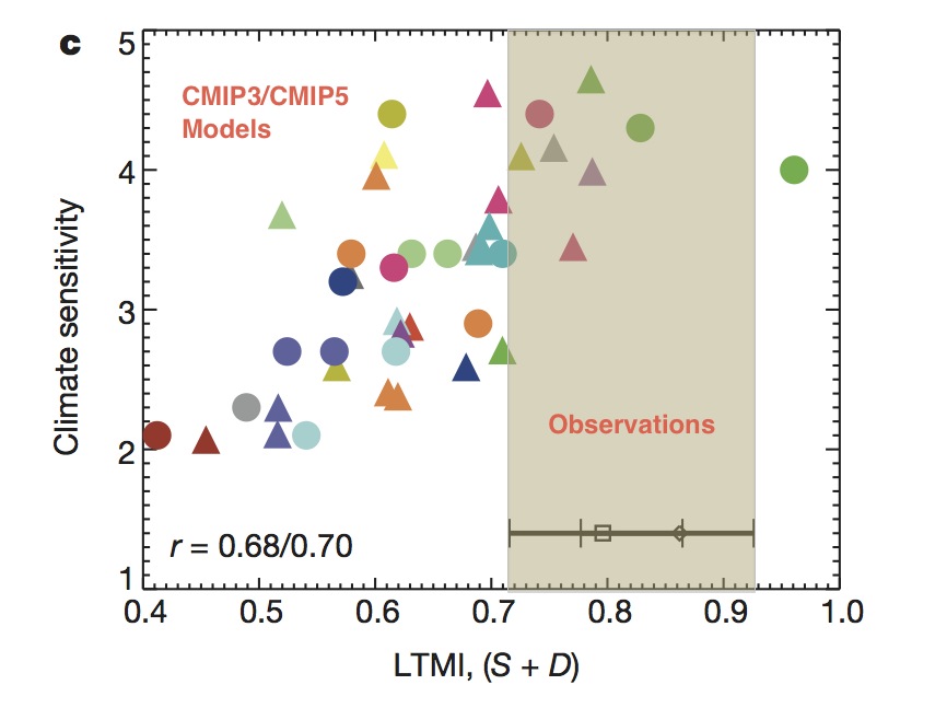
Figure (derived from Sherwood et al, fig. 5c) showing the relationship between the models’ estimate of Lower Tropospheric Mixing (LTMI) and sensitivity, along with estimates of the same metric from radiosondes and the MERRA and ERA-Interim reanalyses.
From that figure one can conclude that this process is indeed correlated to sensitivity, and that the observationally derived constraints suggest a sensitivity at the higher end of the model spectrum.
There was a interesting talk at AGU from Peter Caldwell (PCDMI) on how simply data mining for correlations between model diagnostics and climate sensitivity is likely to give you many false positives just because of the number of possible options, and the fact that individual models aren’t strictly independent. Sherwood et al get past that by focussing on physical processes that have an a priori connection to sensitivity, and are careful not to infer overly precise probabilistic statements about the real world. However, they do conclude that ‘models with ECS lower than 3ºC’ do not match the observations as well. This is consistent with the Fasullo and Trenberth study linked to above, and also to work by Andrew Dessler that suggest that models with amplifying net cloud feedback appear most consistent with observations.
There are a number of technical points that should also be added. First, ECS is the long term (multi-century) equilibrium response to a doubling of CO2 in an coupled ocean-atmosphere model. It doesn’t include many feedbacks associated with ‘slow’ processes (such as ice sheets, or vegetation, or the carbon cycle). See our earlier discussion for different definitions. Second, Sherwood et al are using a particular estimate of the ‘effective’ ECS in their analysis of the CMIP5 models. This estimate follows from the method used in Andrews et al (2011), but is subtly different than the ‘true’ ECS, since it uses a linear extrapolation from a relatively short period in the abrupt 4xCO2 experiments. In the case of the GISS models, the effective ECS is about 10% smaller than the ‘true’ value, however this distinction should not really affect their conclusions.
Third, in much of the press coverage of this paper (e.g. Guardian, UPI), the headline was that temperatures would rise by ‘4ºC by 2100’. This unfortunately plays into the widespread confusion between an emergent model property (the ECS) and a projection into the future. These are connected, but the second depends strongly on the scenario of future forcings. Thus the temperature prediction for 2100 is contingent on following the RCP85 (business as usual) scenario.
Implications
Last year, the IPCC assessment dropped the lower bound on the expected range of climate sensitivity slightly, going from 2-4.5ºC in AR4 to 1.5-4.5ºC in AR5. One of us (Mike), mildly criticized this at the time.
Other estimates that have come in since AR5 (such as Schurer et al.) support ECS values similar to the CMIP5 mid-range, i.e. ~3ºC, and it has always been hard to reconcile a sensitivity of only 1.5ºC with the paleo-evidence (as we discussed years ago).
However, it remains true that we do not have a precise number for the ECS. Sherwood et al’s results give weight to higher values than some other recent estimates based on transient estimates (e.g. Otto et al. (2013)), but it should be kept in mind that there is a great asymmetry in risk between the high and low end estimates. Uncertainty cuts both ways and is not our friend. If the climate indeed turns out to have the higher-end climate sensitivity suggested by here, the impacts of unmitigated climate change are likely to be considerably greater than suggested by current best estimates.
References
- S.C. Sherwood, S. Bony, and J. Dufresne, "Spread in model climate sensitivity traced to atmospheric convective mixing", Nature, vol. 505, pp. 37-42, 2014. http://dx.doi.org/10.1038/nature12829
- J.T. Fasullo, and K.E. Trenberth, "A Less Cloudy Future: The Role of Subtropical Subsidence in Climate Sensitivity", Science, vol. 338, pp. 792-794, 2012. http://dx.doi.org/10.1126/science.1227465
- A.E. Dessler, "A Determination of the Cloud Feedback from Climate Variations over the Past Decade", Science, vol. 330, pp. 1523-1527, 2010. http://dx.doi.org/10.1126/science.1192546
- A.P. Schurer, G.C. Hegerl, M.E. Mann, S.F.B. Tett, and S.J. Phipps, "Separating Forced from Chaotic Climate Variability over the Past Millennium", Journal of Climate, vol. 26, pp. 6954-6973, 2013. http://dx.doi.org/10.1175/JCLI-D-12-00826.1
- A. Otto, F.E.L. Otto, O. Boucher, J. Church, G. Hegerl, P.M. Forster, N.P. Gillett, J. Gregory, G.C. Johnson, R. Knutti, N. Lewis, U. Lohmann, J. Marotzke, G. Myhre, D. Shindell, B. Stevens, and M.R. Allen, "Energy budget constraints on climate response", Nature Geoscience, vol. 6, pp. 415-416, 2013. http://dx.doi.org/10.1038/ngeo1836
“Uncertainty cuts both ways and is not our friend.”
This point can’t be emphasized enough, and all too often is lost in the noise.
How much variance is there in model runs with initial conditions/parameters changed only slightly? Do the spreads in individual model runs grow with larger differing initial conditions?
Thanks
> asymmetry in risk between the high and low end estimates
This needs to be said in fifth-grader language.
Along a line going from lower to higher end temperatures.
— the “long tail” gets thinner — showing the hotter end less likely
— overlay it with a “long club” — showing more damage as it’s hotter
Then you get something like cost-benefit balance.
But look at where we start from now.
Our starting point is, now, already, well into a great extinction at a grossly unnatural rate of change
and we are actively working to make it much worse.
Michael Mann and Gavin Schmidt wrote: “Uncertainty cuts both ways and is not our friend.”
Rob Honeycutt wrote: “This point can’t be emphasized enough, and all too often is lost in the noise.”
Which is, of course, the entire purpose of the noise.
Michael Mann and Gavin Schmidt wrote: “Uncertainty cuts both ways and is not our friend.”
Now run that through the “Science-Talk To Advocacy” translator that the “AGU talk” discussion thread built, and see if there is a way to restate it that is both faithful to the science and also does not leave the listener any room to shrug and say “Yeah, well, so what.”
Authors:
I wonder who the the first denier to quote the highlighted text and say “See! The models are tuned to get the desired output” will be?
Gavin and Mike: Thanks for this well referenced and timely discussion. As you well know this has set off the alarm bells in some circles. Between this and Cowtan and Way, among others, it’s been interesting!
Video: Sherwood explains the new finding in detail.
Peter Sinclair from ClimateCrocks.com noted:
Thanks for covering this important article.
Here is a link to a video featuring Sherwood himself discussing the science and its implications (thanks, prok):
http://climatestate.com/2013/12/31/planet-likely-to-warm-by-4c-by-2100-scientists-warn/
Hank at #3 wrote:
“> asymmetry in risk between the high and low end estimates
This needs to be said in fifth-grader language.”
I may need it in 3rd-grader language. Does the asymmetry just mean that we need to be more worried about uncertainties on the dangerous end than on the safe end because the dangerous end is, well, dangerous.
Or does it mean that there is much less chance of the safer end being real and more reasons to believe that the more dangerous end of the spectrum of possibilities is what we will get? Is there a long, fat tail on high-temperature end of sensitivity estimates and little or no tail on the other side? (Beyond what this one study suggests.)
“…well into a great extinction at a grossly unnatural rate of change
and we are actively working to make it much worse”
Nicely put!
Small typo ” ..and getting that right is a real challenge for climate models.”
[Response: Thanks! – gavin]
Regarding feedbacks, Previdi et al 2013
ESS needs more attention, since this is the sensitivity which includes all feedbacks. Especially so when considering the slow climate inertia. (Which means that with more thresholds we pass, lowering emissions might not help to avert further SLR and large impact associated changes.) Further delay of serious emissions reductions is not an option if we want to keep the current habitability.
Is there some good qualitative explanation for the lower estimate in Otto et al? I suppose that some degree of conflicting evidence is normal in a complex scientific field, but two very different ECS-estimates does not necessarily have to mean a true contradiction in the context of all knowledge, while there are different models used.
Isn’t it true that for the 21st century warming, TCR is the more relevant metric and these ECS revisions do not imply 4C warming as the Guardian article seems to imply?
[Response: As we mentioned, the 4ºC by 2100 is for the RCP85 scenario – basically you take the SPM 7a figure and only look at the top half of the RCP85 temperature responses. Since the multi-model mean warming is around 4ºC (over 1986-2005) by then, the higher sensitivity models will have at least that. To be sure, this is a tad ad hoc, but I think it’s probably accurate enough. As for TCR, you are correct that this is the slightly more relevant metric for near-term projections, but is not what can be constrained directly with this analysis. – gavin]
From just thermodynamics, one can imagine that the mean cloud density occupies a position in the P-V-T (Pressure-Volume-Temperature) phase space, or equivalently Pressure-Density-Temperature. And as temperature increases, if the P-V-T steady-state is to be maintained, the “average” cloud will need to increase in altitude, largely due to the properties of the atmospheric lapse rate.
Increasing in altitude, the character of the cloud may also change subtly, as ice-clouds are more prevalent at higher altitudes.
How often are these simple first-order physics principles applied?
So what happens if you use the Sherwood et al parameters on those models with a lower sensitivity and re-run the 20th century back cast?
It looks like you are going to get a running average model mean well above the actual global temperatures at the end of the century and given the divergence in modelled output from reality in this century then there will be a good chance that they would already be falsified.
Would this be a good thing?
Alan
I’ve been critical of what I’ve considered excessively low estimates of climate sensitivity such as those found in Otto et al, for reasons including the inaccuracy of forcing estimates, the disparity between recent planetary warming (as shown by ocean heat uptake) and surface warming, and the cool bias introduced by equating “effective climate sensitivity” with ECS as conventionally defined on the basis of Charney type feedbacks. On the other hand, having struggled through this paper, I have some reservations about accepting its much higher estimates without further supporting evidence. In particular, I wondered whether to some extent, it didn’t assume what it set out to prove. Specifically, if increased lower tropospheric mixing does in fact dry the boundary layer and reduce low cloud cover, then it should in fact imply a strong positive cloud feedback and hence high ECS. Consequently, observations supporting increased mixing would imply higher sensitivity and models that reproduced these observations would be characterized by higher ECS values. But does this mechanism operate as presumed? If the reality is more complex than a simple case of increased mixing causing boundary layer drying and diminished cloudiness, then the concordance of high ECS models and observed evidence for mixing would not necessarily translate into a specific range of ECS values. (I would also add that the evidence for the increased mixing was rather indirect, but I don’t feel qualified to judge the adequacy of those data).
Based on the above, my reaction to the paper was, “It’s plausible, but is it true?” What I would hope for is further discussion by those with expertise in this area explaining why the arguments in the paper shouldn’t be considered more than a reasonable hypothesis consistent with the evidence but not yet strongly confirmed by it. I’m comfortable with arguments for ECS values exceeding 2 C, but not yet ready to judge them greater than 3 C without further reasons for doing so.
The Hansen prognosis based on empirical and paleo-climate evidence that climate sensitivity is ~3C and with BAU, likely to be achieved by mid century. Now we appear to have another line of evidence from Sherwood et al. supportive of this.
Gavin/Mike- What I’ve been struggling with in Sherwood et. al. is:
If the evaporated water isn’t making it up to 15 km, and downdrafts of dry air from above disperse it, blocking low cloud formation…how eventually does the water vapor precipitate out? I’ve not been able to puzzle this out from you notes, Sherwood’s talk or the article itself. For hydrological balance it’s got to come out somewhere, sometime, and make some clouds, and those need to show up in the models at the right altitude and albedo/IR absorbing effect.
“ECS is the long term (multi-century) equilibrium response to a doubling of CO2 in an coupled ocean-atmosphere model. It doesn’t include many feedbacks associated with ‘slow’ processes (such as ice sheets, or vegetation, or the carbon cycle).”
Some of these feedbacks seem not so slow ? albedo flip from arctic sea ice for example ? or Greenland darkening ? Anybody try decreasing those time constants, just for fun ?
“Thus the temperature prediction for 2100 is contingent on following the RCP85 (business as usual) scenario.”
Does anyone seriously think (as opposed to “hope”) that BAU will not continue for as long as it can? From what I can make out of government inaction, talk and get rich carbon schemes, the only thing that will stop BAU is resource scarcity (including of fossil fuels), economic disruption from climate change (and other environmental degradation), or societal disintegration (from the impacts of resource scarcity and environmental degradation). So, techno-optimists and wishful thinkers will actually want BAU and should prepare for 4C rise by 2100 (which means a dangerous rise well before that, with more later). The rest of us will hope that the industrial civilisation breaks down quickly enough to keep parts of the planet habitable.
“Mixing is associated with reductions in low cloud cover”–this seems counter-intuitive. Why doesn’t more mixing of water vapor in the lower troposphere create _more_ low altitude (cooling) clouds?
There is something basic that I seem to be missing here. Clarity from any direction would be greatly appreciated.
wili, the term “updraft” might explain this better.
The analysis assumes that the only difference between models affecting ECS are low clouds. But is that actually true ? There are also similar spreads in model values for water vapor and lapse rate feedbacks. (Bony et al.)
[Response: not really. The correlation btw ECS and LTMI makes no such assumption. There is of course spread which will be associated with other issues, but cloud feedbacks are the ones with largest spread. – gavin]
I saw a comparison from 1980 to present, which compared the observed trend against each AR5 model trend (made up of all the runs from each model). This seemed to show the observed trend was right at the bottom (or even below) even the least sensitive models.
I thought 1980 to present was probably long enough for the long term forced trend to emerge.
How would it be possible to reconcile this trend with the more sensitive models ? (I did read the excellent recent rc models vs obs post)
I thought maybe mis estimates of the forcing, some problems with measurements (although I thought surface temperature trends were pretty well sorted )
I wondered if the cloud feedback varied over time or maybe the models TCR was too high.
If the TCR did indeed turn out to be lower than expected but the ECS was unaffected, would that really be that reassuring ? Surely it just means that there is more hidden warming in the pipeline that we have limited opportunity to affect ?
Isn’t it possible that models with higher ECS’s can better match “observations” in a cloud context, but at the same time be a worse match for “observations” in a surface temperature context?
If that’s the case, what does that mean then..? Such a discovery gives us little solace because we still don’t have a good handle on cloud impacts anyway, and the more important contexts for policy has always regarded getting accurate temperature projections/expectations rather than accurate mid/high level cloud expectations. No?
[Response: Model/observation mismatches can have many causes. You can’t assume the answer ahead of time. – gavin]
Mike and Gavin, Thanks for this. Back when the AR5 downshifted the lower climate sensitivity bound, I took a look at the estimates and found that the distribution of estimates as given on the AGW Observer site seemed to be bimodal:
http://agwobserver.wordpress.com/2009/11/05/papers-on-climate-sensitivity-estimates/
The two modes seem to be centered ~2.1 and 3.5 degrees per doubling. What is more, it appears that the shorter the equilibrium time assumed or implied, the lower the sensitivity estimate. Given that a lot more energy seems to be going into the oceans than we thought (mixing results), this would seem to imply a longer time to return to equilibrium after a perturbation, and so a higher sensitivity. Do you know of any work that has been done on this, or do you have any insights? Thanks.
> how eventually does the water vapor precipitate out?
Mysterious atmospheric rivers?
Nobody knew about these at all til a few years ago.
Apparently what flooded Colorado arrived as very humid air, not as clouds ….
uh, yep: http://iopscience.iop.org/1748-9326/8/3/034010/article
David A Lavers et al 2013 Environ. Res. Lett. 8 034010
doi:10.1088/1748-9326/8/3/034010
Future changes in atmospheric rivers and their implications for winter flooding in Britain
@25. Model/observation mismatches can have many causes. You can’t assume the answer ahead of time. – gavin]
When it comes to assessing the future 2100 Global Temperature Anomaly value, and as part of that establishing the ECS value of Carbon, wouldn’t:
Studies that show ECS values that match “temperature” observations > Studies that show ECS values that match “cloud” observations ?
Given that it’s still an active research question as to what actually causes mismatches, absent anything definitive wouldn’t a theoretically balanced distribution of possibilities thus still converge on the above result?
[Response: I have no idea what you are asking. However, we said in the top post that the one needs to reconcile all of the evidence (paleo, climatological, transient) to get a robust result. Right now that ends up at around 3ºC – but there is still work to do to make these constraints be as comparable as they could be. – gavin]
“A new paper … suggests that models with an equilibrium climate sensitivity (ECS) of less than 3ºC do much worse at fitting the observations than other models… the impacts of unmitigated climate change are likely to be considerably greater than suggested by current best estimates.”
Logic told us this years ago. I posted here (Likely as ccpo) long ago that the disconnect between magnitude of effects in the real world and assumptions about lower sensitivity were a clear indication that sensitivity *had* to be higher. At the time @ 2006-7, the key incongruities were ASI melt and Antarctica melting already getting underway. In 2007 we had a huge ASI melt, the report about the thermokarst lakes tripling from around 2000 – 2007. These reports alone strongly reinforced the idea sensitivity was being underestimated.
Hopefully, you all will start considering considerations other than science papers. Systems analysis plays a role here, and beat you guys to the punch by seven years. That’s a lot of lost time in a rapidly debilitating world.
> systems analysis
Look back a bit and you’ll find this is part of the ongoing discussion, e.g. 17 Jul 2006 at 6:06 PM
Recent news:
http://www.iiasa.ac.at/web/home/about/news/20131216-ISIMIP.en.html
International Institute for Applied Systems Analysis
17 December 2013
Thanks (again) prok. So the mixing is so low and rapid that it doesn’t really form the low clouds?
Interesting point on atmospheric rivers, Hank.
Welcome back, Killian/ccpo.
Hank- Thanks very much for the atmospheric rivers concept. you could use the geographic concentration to then argue for minimal climatic effects of the clouds, maybe? Smaller footprint radiative forcing wise for the amount of water vapor?
> you could use the geographic concentration to then argue …
Oh, no, not me.
I’m going to wait for the scientists on these questions, not argue.
It’s the same planet; the clouds are the same clouds. The moisture moves from one place to another — now we know something more about how it moves, that’s all.
Wili, i still read about clouds but this here helped me to better understand the physical processes at work http://www.ldeo.columbia.edu/~martins/climate_water/lectures/evap_precip.htm It appears to depend on many factors like as above mentioned the type of cloud or water vapor pressure (see the figure from columbia link) or if a condensation nuclei is present.
I found out you can actually access the study paper at nature directly with preview access (ReadCube).
Gavin: Is the trouble with atmospheric rivers (ARs) is that they are spatially small and hard to model with a GCM? And also hard to relate to GW for the public? But:
“Future changes in atmospheric rivers and their implications for winter flooding in Britain”
“3. Results and discussion”
“It is therefore evident that the CMIP5 models are capable of resolving AR-like structures”
But ARs could be a lot smaller, couldn’t they?
Gavin: AR doesn’t mean “storm track” does it? The paper mentions “storm track” and then ARs are something different. But an AR could be mistaken for a storm by a weather forecaster? So weather forecasters need a course in ARs. Figure 1 doesn’t look like a hurricane at all. The AR is long and thin, not a circle.
Another scary thing about GW: Nobody is safe from floods or mega-snowstorms. We can protect ourselves from the usual, but ARs are a whole new hazard. As in: I live at the top of the bluff where flooding seems to be impossible, I thought and I hope.
I am asking for RC to do an article on ARs. Maybe a research program.
The Guardian’s version might be slightly confusing to beginners; it stated:
I think it would have been clearer to have explicitly mentioned the third process i.e. the formation of low clouds which should be reduced in amount by the second process (‘drifting back down’). These low level clouds are expected to have a net cooling effect unlike the high ones mentioned in the quotation.
[With apologies to Damian Carrington but his article is now closed for comments.]
Hank #3 wrote:
>> asymmetry in risk between the high and low end estimates
> This needs to be said in fifth-grader language.
I like Richard Alleys car example. Let’s say you’re planning a road trip. What do you expect? You get stuck in traffic for some time and the radio plays bleh tunes. If it’s a good day, there’s little traffic and the radio plays a beach boys concert [his music choice :-)]. On a bad day, there’s lots of traffic and on the radio they’re testing the emergency broadcast system.
But what do we actually prepare for? Safety belts, crumple zones, airbags, donations to mothers against drunk driving… Nobody goes on the road expecting an accident but we do a lot to prepare for it.
It should be the same with climate. Even if we don’t expect the worst, we should be prepared for it.
> But ARs could be a lot smaller, couldn’t they?
Why would you think so?
Look at the pictures: http://www.meted.ucar.edu/norlat/sat_features/ars/media/graphics/AR_Global_IWV_Dec_28_2011_feedback.jpg
Below some size, it’d break up (or we’d call it something else).
Look with Scholar and you’ll find papers modeling ARs with various grid sizes (increasingly finer resolution) testing the limits of what’s useful.
also
> Another scary thing …
> ARs are a whole new hazard.
Not so. Not at all.
We’ve known these hazards from even the very short few centuries of history we have, e.g.:
https://en.wikipedia.org/wiki/Great_Flood_of_1862
Plus more and better paleo records, e.g.
http://www.ncdc.noaa.gov/paleo/globalwarming/paleodata.html
Putting a name (“Atmospheric river”) to what’s happened doesn’t create a new hazard. It helps explain a hazard we knew existed.
Putting a name on it shouldn’t make it more scary.
November 15, 2013 Study Uses NASA ‘A-Train’ to Measure Atmospheric River Properties
As pointed out, the 4C by 2100 does represent a “business as usual” approach to our carbon emissions, but also a business as usual approach to the uptake of a generous portion of those emissions by the ocean. Should some threshold be reached in which the ocean no longer takes up as much carbon, we could see higher temperatures.
Dave @ 18 asks more or less: When & where does the rain fall, and where have all the clouds gone?
Then the discussion went to atmospheric rivers. It is nice to learn more about them, but getting back to Dave’s question:
Most evaporation occurs at sea and most rain falls there too.
Relative humidity has stayed about the same as before even while temperatures are a bit higher. Does this cause about the same rate of evaporation as before, or is there more evaporation on an average day now with a vapor molecule residing in the air for less time?
One thing I have heard is that on land, wet areas are getting wetter (more rain) and dry areas are getting drier, and more rain inches fall in brief torrents, with longer rainless days in between, than before. An increase in atmospheric rivers would fit this pattern but would be only the most dramatic part of it.
So part of the answer to Dave’s question may be that rain falls for less time but in more torrents. Does this hold water?
The West Coast’s Pineapple Express occurs during the normal rainy season, November through February. The storms that caused flooding in Colorado and New Mexico this year arrived in September, overlapping the annual monsoon season of July and August. I wonder if that means anything?
Thinking about my own question, the common factor appears to be humid tropical air being entrained by extra-tropical cyclones, something that’s already been observed about ARs.
#44–The AR5 Technical Summary also points out that while roughly constant mean global RH has been observed and may not be too far from the case in the future, there is expected to be spatial structure to RH as warming proceeds: over land we expect to see drying areas experiencing lower RH (and perhaps the converse as well). I’m paraphrasing from memory here; hopefully I’m not distorting too much in the process.
“Look back a bit and you’ll find this is part of the ongoing discussion”
Yes, Hank, I’ve been one of those pushing it. And, no, the breadth of analysis yet available is still not being used. Why do you think my assumptions have been mor eaccurate over the last 7 years? Sheer luck over that long a time frame?
Thanks for chiming in. Add something next time?
In the paper a positive tropical cloud feedback is postulated which leads to CS 4…5. (see also: http://www.eurekalert.org/pub_releases/2013-12/uons-ncs121913.php with the headline “Cloud mystery solved: Global temperatures to rise at least 4°C by 2100″). Anyway, in the paper is not too much empirically evidence from observations included. So I tried this one: Have a look at fig. 3 and 4 where the you can see that the lower altitude drying effect is located at an area -30…30N over the oceans. So I looked at the SST ( HadISST1) of the IPWP ( see fig. 1) and found, that the saisonal variation is about 1 K between May ( max.) and August ( min). If the “Sherwood-effect” is at work one should assume that the slope of the SST- trend of Aprils is higher than the slope of the SST- trend of Augusts over the years 1975…2013 due to the positive feedback presumed in the paper. This is not the case: http://www.dh7fb.de/reko/ipwpdelta.gif . The difference between the (warmer) May-SST and the (colder) August-SST is very slightly ( not significant) negative correlated with the SST of the May. In my eyes this observation is not a hint for a positive cloud feedback?
> do you think my assumptions have been
> mor eaccurate over the last 7 years?
I couldn’t say, as I don’t recollect anything from you back then.
For accuracy, Hansen in 1986 is the gold standard, I’d say:
http://babel.hathitrust.org/cgi/pt?id=mdp.39015035756843;view=1up;seq=1
“Jump to” 18 at the bottom of the page and read forward
(pointer from one of Gavin’s tweets)
In hindsight, he got on record what we needed to know then.